7.10 bunched_beam_moments

• type: setup command.
• sequence: must follow run_control.
• function: set up for tracking of particle coordinates with various distributions.
• Command syntax, including use of equations and subcommands, is discussed in 7.2.
• Notes:
  • In Pelegant, the exact particles generated will change as the number of cores is changed.
  • This command is used when it is convenient to specify the beam dimensions in terms of beam sizes, divergences, and other moments. The bunched_beam command can be used when it is more convenient to specify lattice functions, emittances, etc.

• bunch — The (incomplete) name of an SDDS file to which the phase-space coordinates of the bunches are to be written. Recommended value: “%s.bun”.
• n_particles_per_bunch — Number of particles in each bunch.
• multiply_np_by_cores — If non-zero, the number of particles is multiplied by the number of working cores.
• time_start — The central value of the time coordinate for the bunch.
• matched_to_cell — The name of a beamline from which the Twiss parameters of the bunch are to be computed.
• use_moments_output_values — If nonzero, then the beam is generated to match the 6D matched, equilibrium beam moments computed by the moments_output command. The distribution type must be gaussian. This mode is incompatible with using closed orbit correction with start_from_centroid=1 (the default value).
• Po — Central momentum of the bunch.
• S1_beta, S2_beta, S3_beta, S4_beta — Horizontal beam size and divergence, vertical beam size and divergence, for betatron coordinates. For example, for the x coordinate, we have

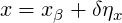  (3)

  where x_β is the betatron component, δ is the fractional momentum deviation, and η_x = Σ₁₆∕Σ₆₆.

• S5 — Fractional energy spread.
• S6 — Fractional bunch length.
• S56 — Σ₅₆.
• Sij_beta — Element of the beam sigma matrix for betatron coordinates.
• spin — Provide the components of the spin vector to use for all particles. Ignored if spin_tracking=0 in run_setup. The vector is normalized to have unit magnitude.a
• one_random_bunch — If non-zero, then only one random particle distribution is generated. Otherwise, a new distribution will be generated for every simulation step.
• enforce_rms_values[3] — Flags, one for each plane, indicating whether to force the distribution to have the specified RMS properties.
• distribution_cutoff[3] — Distribution cutoff parameters for each plane. For gaussian distributions, this is the number of sigmas to use. For other distributions (except dynamic aperture), this number simply multiplies the sizes. This is potentially confusing and hence it is suggested that the distribution cutoff be set to 1 for nongaussian beams.

  The exception is “dynamic-aperture” distribution type. In this case, the cutoff value is the number of grid points in the dimension in question.

• distribution_type[3] — Distribution type for each plane. May be “gaussian”, “hard-edge”, “uniform-ellipse”, “shell”, “dynamic-aperture”, “line”, “halo(gaussian)”.

  For the transverse plane, the interpretation of the emittance is different for the different beam types. For gaussian beams, the emittances are rms values. For all other types, times the distribution cutoff defines the edge of the beam in position space, while times the distribution cutoff defines the edge of the beam in slope space.

  A hard-edge beam is a uniformly-filled parallelogram in phase space. A uniform-ellipse beam is a uniformly-filled ellipse in phase space. A shell beam is a hollow ellipse in phase space. A dynamic aperture beam has zero slope and uniform spacing in position coordinates. A line beam is a line in phase space. A “halo(gaussian)” beam is the part of the gaussian distribution beyond the distribution cutoff.

• limit_invariants — If non-zero, the distribution cutoffs are applied to the invariants, rather than to the coordinates. This is useful for gaussian beams when the distribution cutoff is small.
• limit_in_4d — If non-zero, then the transverse distribution is taken to be a 4-d gaussian or uniform distribution. One of these must be chosen using the distribution_type control. It must be the same for x and y. This is useful, for example, if you want to make a cylindrically symmetric beam.
• symmetrize — If non-zero, the distribution is symmetric under changes of sign in the coordinates. Automatically results in a zero centroid for all coordinates.
• halton_sequence[3] and halton_radix[6] and optimized_halton — This provides a “quiet-start” feature by choosing Halton sequences in place of random number generation. There are three new variables that control this feature. halton_sequence is an array of three flags that permit turning on Halton sequence generation for the horizontal, vertical, or longitudinal planes. For example, halton_sequence[0] = 3*1 will turn on Halton sequences for all three planes, while halton_sequence[2] = 1, will turn it on for the longitudinal plane only.

  halton_radix is an array of six integers that permit giving the radix for each sequence (i.e., x, x’, y, y’, t, p). Each radix must be a prime number. One should never use the same prime for two sequences, unless one randomizes the order of the sequences relative to each other (see the next item). If these are left at zero, then elegant chooses values that eliminate phase-space banding to some extent. The user is cautioned to plot all coordinate combinations for the initial phase space to ensure that no unacceptable banding is present.

  A suggested way to use Halton sequences is to set halton_radix[0] = 2, 3, 2, 3, 2, 3 and to set randomize_order[0] = 2, 2, 2,. This avoids banding that may result from choosing larger radix values.

  optimized_halton uses the improved halton sequence [33]. (Algorithm 659, Collected Algorithm from ACM. Derandom Algorithm is added by Hongmei CHI (CS/FSU)). It avoids the banding problem automatically and the halton_radix values are ignored.

• randomize_order[3] — Allows randomizing the order of assigned coordinates for the pairs (x, x’), (y, y’), and (t,p). 0 means no randomization; 1 means randomize (x, x’, y, y’, t, p) values independently, which destroys any x-x’, y-y’, and t-p correlations; 2 means randomize (x, x’), (y, y’), and (t, p) in pair-wise fashion. This is used with Halton sequences to remove banding. It is suggested that that the user employ sddsanalyzebeam to verify that the beam properties when randomization is used.
• centroid[6] — Centroid offsets for each of the six coordinates.
• first_is_fiducial — Specifies that the first beam generated shall be a single particle beam, which is suitable for fiducialization. See the section on “Fiducialization in elegant” for more discussion.
• save_initial_coordinates — A flag that, if set, results in saving initial coordinates of tracked particles in memory. This is the default behavior. If unset, the initial coordinates are not saved, but are regenerated each time they are needed. This is more memory efficient and is useful for tracking very large numbers of particles.